Yield Line And Fe Load Decomposition With Example


- When slab and beams are modelled, the slab load is automatically calculated by default using yield-line tributary area method.
- All the slab line / point load will be converted to equivalent area load. Hence, although the total load is captured by the beam, the localized effect of these loads cannot be evaluated.
- All slab openings are ignored. Hence if there are large slab openings, the loadings on the beams will be conservative.
- Suitable for regular rectangular or squarish slabs. May not be sufficient for irregular shaped slabs.
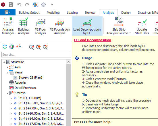
- Run by going to Loading (top menu) or Analysis (top menu) > Load Decomposition by FE
- This is an alternative to the default “Yield Line” slab load calculation onto beams
- The localized effect of concentrated slab loads can be considered because the slabs are meshed
- Slab opening is considered, i.e. slab loads decomposed onto beam with slab openings will be different.
- Should be used when there are many irregular shaped slabs (non rectangular or squarish slab)
- This method consumes more time in analysis compare to yield line tributary area method, in order to mesh slabs into plates and shells especially large number of slabs to be meshed in the model.

What is Load Decomposition?
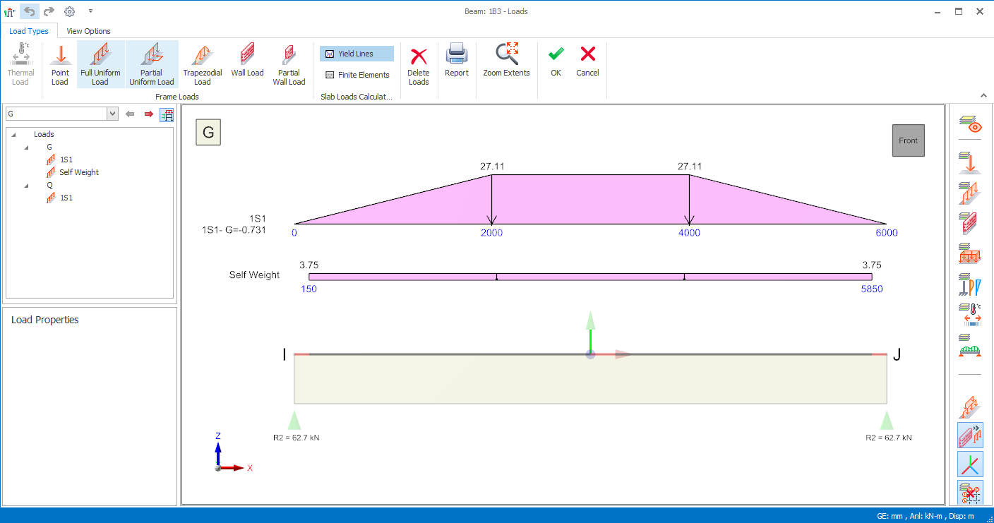
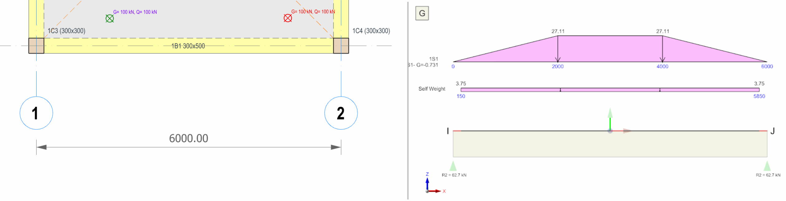
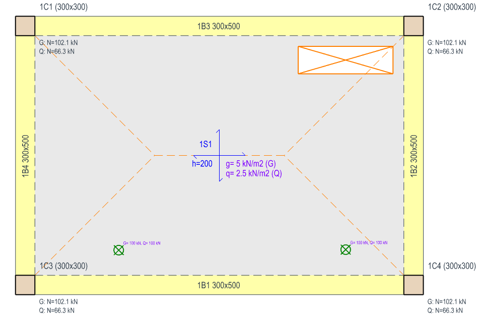
The boundaries of the tributary areas loading each beam can be viewed graphically as shown above. These look similar to potential Yield Lines, hence the name given to this default method.
In this, as in many other areas, ProtaStructure effectively applies the sort of engineering methodology that has been used in hand calculations for many years.
Why switch to a FE method?
Yield Lines method has limitations in circumstances such as:
- When the slab boundaries are highly irregular and particularly where some edges of a complex boundary are unsupported.
- When there are significant holes defined in the slab.
- When there are eccentric concentrated point, patch, or line loads.
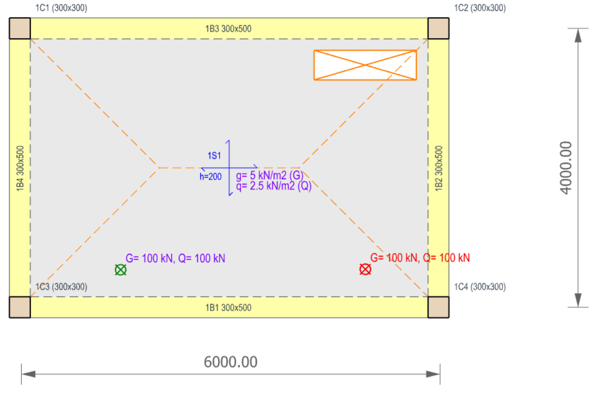
Example of FE Method for Slab Load Decomposition
By using the optional Finite Elements Model, the point loads will be much more accurately distributed. The slab load will also be more accurately distributed, including the deductions and effects associated with the void.
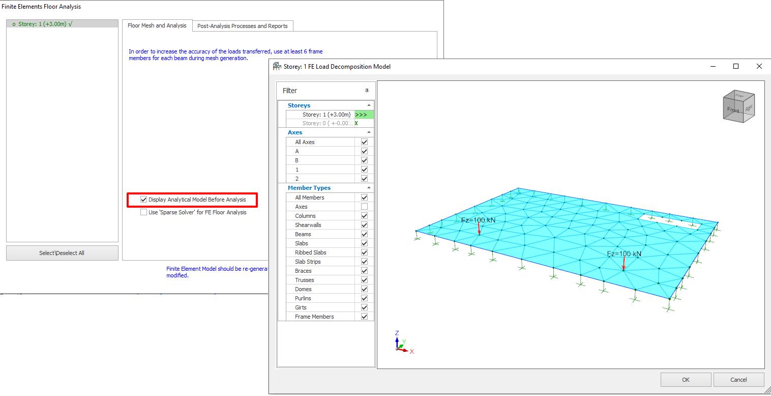
1. Select the Load Decomposition by FE command from the Loading menu as shown below.
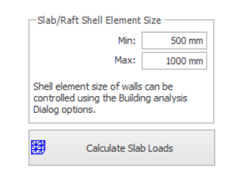
On the left panel, select the storey first, then click on the button "Calculate Slab Loads" to perform FE Load Decomposition analysis.
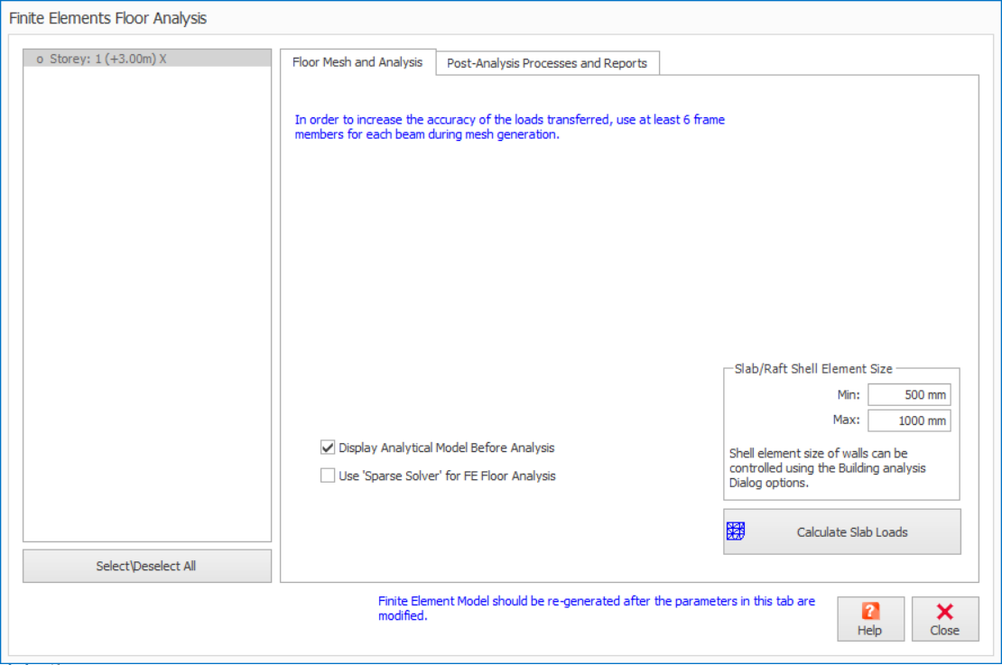
2. Minimum of 500 mm and Maximum of 1000 mm for Slab Shell Element Size are suggested by default, however you can adjust these values.
3. Click the "Calculate Slab Loads" button and the slab is meshed automatically for the selected/ all storeys.4. Check for "Display Analytical Model Before Analysis” to view at the generated mesh for each floor.
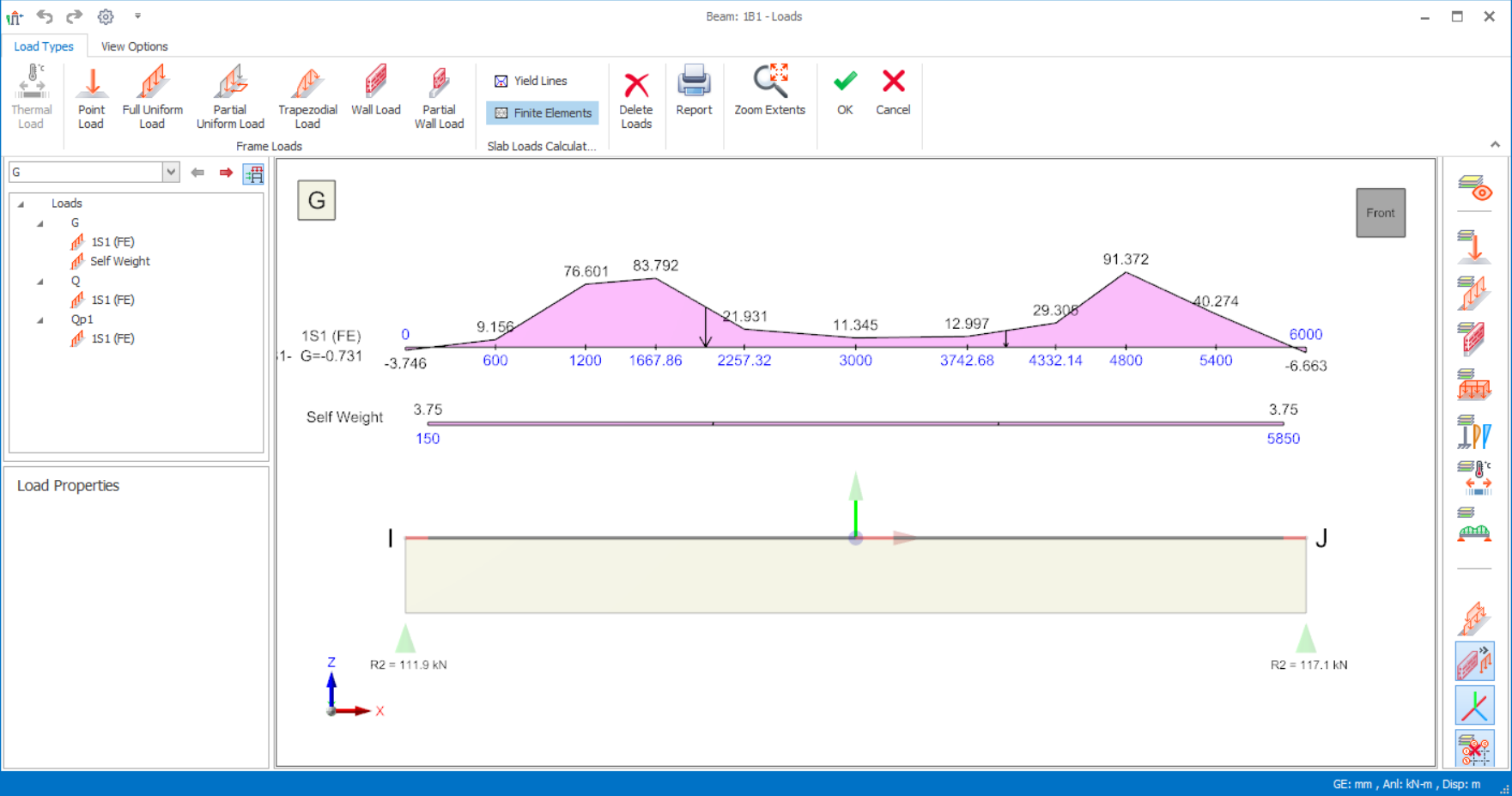
- A dummy support is auto inserted at each beam segment node. This means the beam cannot deflect. Hence, the beam stiffness has no effect on the slab load transfer.
- Slab load is decomposed or calculated only at the beam segment nodes :
- Too few slab meshes will mean lower accuracy, as loading are assumed to be linear between nodes.
- Too many meshes means analysis time is unnecessarily long, especially when the slab layout area is large.
- The general guideline is 6 to 8 meshes along each supporting beam.
- In this case, the suggested slab shell element size results in minimum 8 nodes along each beam; and although not well meshed around the opening this is probably sufficient in this simple example for the intended purpose.
To utilise these new loadings it is necessary to reperform the building analysis. On completion we can see a very different distribution of column loads.
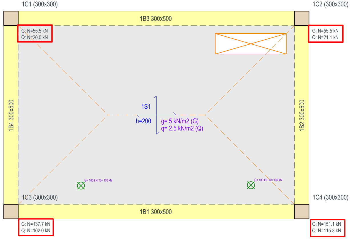
The total Imposed Load using the Yield Line method was approximately 266.4 kN. Using the FE method, it has dropped to 258.4 kN, this is slightly lower because no load is applied to the hole.
 If you change any slab loads or beam layouts, you must remember to reperform the Load Decomposition by FE command before reperforming the building analysis.
  Axial load comparisons are performed at the end of each analysis. This is a comparison of applied loads vs. analysis reactions. Since you can choose decomposition methods on a beam‐by‐beam basis you can cause this comparison to show discrepancies. In the example above, if you choose finite element decomposition for beam 1B1 only, the comparison will be displayed as shown below.
 Why retain the traditional yield line method?
 In the FE method beams are replaced by a line of fully fixed supports. As a consequence, in ordinary regular slabs both the yield line and FE method will share loads equally to internal and edge beams. In other words continuity is not being considered. This is a simplification that has long been accepted in hand calculations.
A more extreme example of the above would be a cantilever slab. The beam adjacent to the cantilever takes the entire cantilever slab load, plus half of the internal slab load, for long cantilevers that can be a significant under estimate.
The only way to account for continuity in such a case would be to include the floor slabs by meshing with Building Analysis, by checking option Include Slabs in Building Model in Building Analysis > Slab Model dialog. This method deals with the continuity, a higher load is put on the beam adjacent to the cantilever and correspondingly less load is put on the next internal beam ‐ some engineers may prefer this.
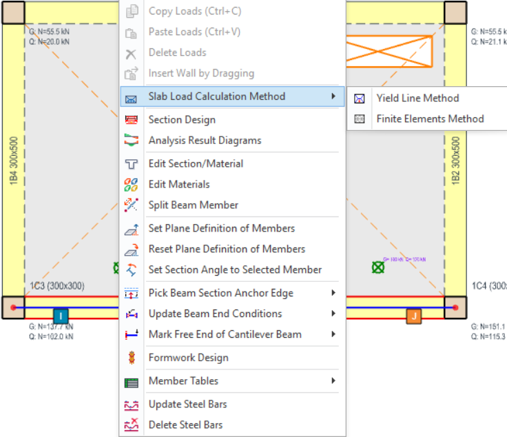
How to switch back to the traditional (yield line) method from FE Load Decomposition method?
- Right click any beam (regardless of 2D view or 3D view)
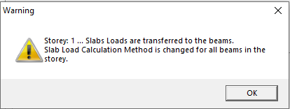
- Click Slab Load Calculation Method
- Select Yield Line Method
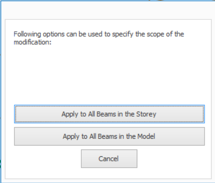
-
- This option can be applied to all beams in the storey or all beams in the model.